The appeal of an implicit function to model a bouncing object first came when creating the graphs at /tools/graphs/. Lets say you have a GUI element you want to bounce into view, for example the high scores at the end of a game. You could create and store a global $y$ position, model velocity and acceleration, deal with fixed/non-fixed time steps etc. Rather than do that for every item, wouldn’t it be great to have a single interpolation function: given a time $t$, what height is my bouncing thing?
Imagine you have a ball that starts on the ground with an initial velocity. For a short time the $y$ position can be nicely modelled with a simple quadratic:
That is, zero initial position, $v$ starting velocity and gravity $g$, which is negative. This works great as the ball flies up, slows, and falls back down just like Newton discovered. The problem is there’s nothing to model a collision with the ground again, and a repeated bounce, and another collision etc. Normally there would be a check that looks something like this:
if (y < 0)
    v = -v;
This should be modelled by a bounce function. There’s also some approximations made which could be improved by an implicit bounce function. Firstly, y < 0, so the ball is below the ground. In reality it would have hit the ground and started moving upwards. y = -y; would be a good start, but since the true collision at y == 0 it’s still been accelerating downwards when it should have been de-accelerating while moving up. Also, v = -v; produces a perfectly elastic collision where no energy is lost. At the time of the bounce, the velocity should also be scaled by a coefficient of restitution: v = -c * v;.
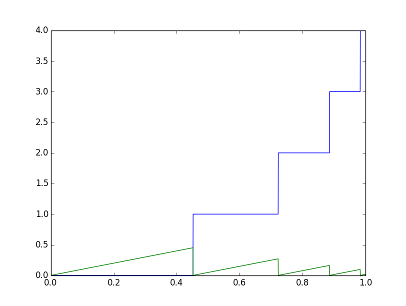
The first thing needed is $n$, an integer that counts bounces as time $t$ increases. Now rather than $v$, the initial velocity of each bounce can be set to $c^n v$ to model successive bounces. Then we just need the time since the start of each bounce $t_b = t - t_n$, and we can create a finished product:
The following image plots $n$ and $t_b$ to show how they separate the components of each quadratic bounce.
OK, so there’s still a few things left to do, namely defining $n$ and $t_b$. A tricky part in doing so is that not only does the the height of successive bounces decrease, but so does the duration of each bounce.
The duration $d$ a bounce takes to complete is found by the difference in roots of the quadratic equation above, using the quadratic formula with $a=\frac{g}{2}$, $b=c^n v$ and $c=0$. The absolute of gravity is taken so as not to give a negative $d$.
Now that the duration of each bounce is known, the absolute time $t_n$ at the start of each bounce is given by the following recurrence relation:
Finally, we have a relationship between $t$ and $n$. It just needs to be inverted:
Note that this function asymptotes as the ball bounces to a stop, producing the log of a negative. So as input use $\min(t, t_{10})$ for example to limit the number of bounces to 10. This cancels, but due to the scale by $g$ which is negative, the $min$ changes to a $max$. Putting it all together, and substituting:
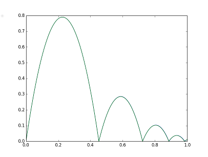
Finally, there exists a single function to model a bounce. Below is a plot of $y(t)$ created with with $v=7$, $c=0.6$ and $g=-31$. Its green line nicely covers a blue numerical solution for validation, using the midpoint method and the collision approach discussed above.